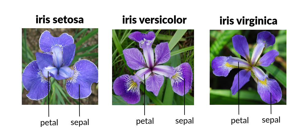
This is a quick exercise using a classic dataset from 1936. This data set contains measurements of the petals and sepals of three different varieties of Iris flowers: Iris Setosa, Iris Versicolour, or Iris Virginica. The objective is to use the decision tree algorithm to train the model to classify the entries into the tree types of Iris.
import numpy as np # linear algebra
import pandas as pd # data processing, CSV file I/O (e.g. pd.read_csv)
from sklearn.model_selection import train_test_split
from sklearn.tree import DecisionTreeRegressor,plot_tree
import matplotlib.pyplot as plt
import seaborn as sns

import warnings # To suppress some warnings
# Suppress the specific FutureWarning
warnings.filterwarnings("ignore", category=FutureWarning, module="seaborn")

df=pd.read_csv('/kaggle/input/iris-flower-dataset/IRIS.csv')
I start on getting the basic info on the dataset
df.info()<class 'pandas.core.frame.DataFrame'> RangeIndex: 150 entries, 0 to 149 Data columns (total 5 columns): # Column Non-Null Count Dtype --- ------ -------------- ----- 0 sepal_length 150 non-null float64 1 sepal_width 150 non-null float64 2 petal_length 150 non-null float64 3 petal_width 150 non-null float64 4 species 150 non-null object dtypes: float64(4), object(1) memory usage: 6.0+ KB
Are there any null entries?
df.isnull().sum()
sepal_length    0
sepal_width     0
petal_length    0
petal_width     0
species         0
dtype: int6
Now I would like to see more about the data on the columns, its central tendency, minimum and maximum values, as well as quantiles
df.describe()| sepal_length | sepal_width | petal_length | petal_width | |
|---|---|---|---|---|
| count | 150.000000 | 150.000000 | 150.000000 | 150.000000 |
| mean | 5.843333 | 3.054000 | 3.758667 | 1.198667 |
| std | 0.828066 | 0.433594 | 1.764420 | 0.763161 |
| min | 4.300000 | 2.000000 | 1.000000 | 0.100000 |
| 25% | 5.100000 | 2.800000 | 1.600000 | 0.300000 |
| 50% | 5.800000 | 3.000000 | 4.350000 | 1.300000 |
| 75% | 6.400000 | 3.300000 | 5.100000 | 1.800000 |
| max | 7.900000 | 4.400000 | 6.900000 | 2.500000 |
Next, I just want to visualize how many entries for each type of Iris there is in the dataset
plt.figure(figsize=(8,4))
sns.countplot(data=df, x='species', palette='RdPu')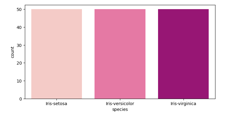
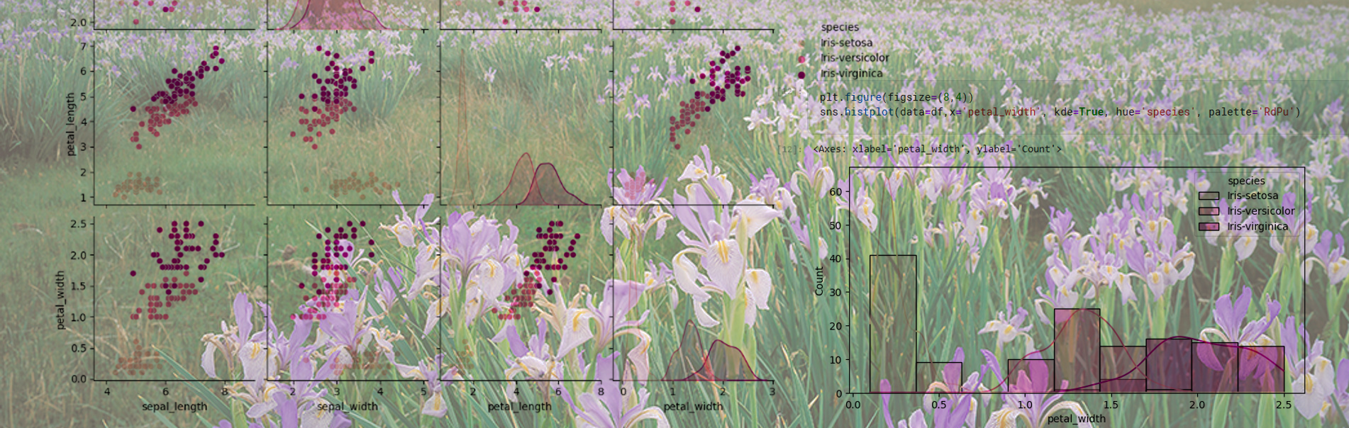
Next I visualize the distribution of the measured data of the flowers
Starting with the petal width. Soon we see that Iris setosa is easier to differentiate from the other two Irises
plt.figure(figsize=(8,4))
sns.histplot(data=df,x='petal_width', kde=True, hue='species', palette='RdPu')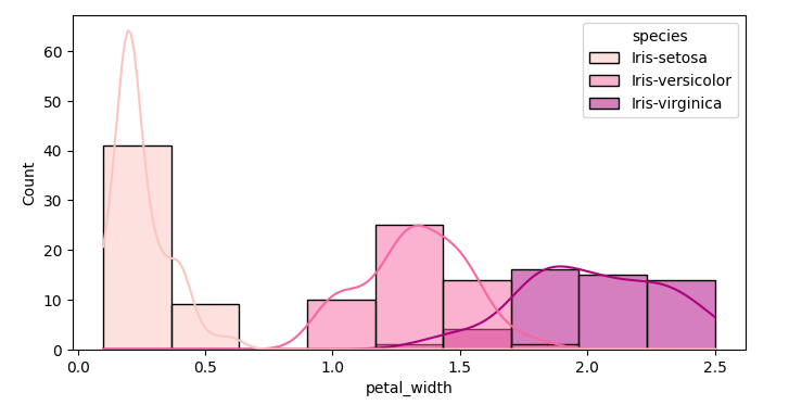
plt.figure(figsize=(8,4))
sns.histplot(data=df,x='petal_length', kde=True, hue='species', palette='RdPu')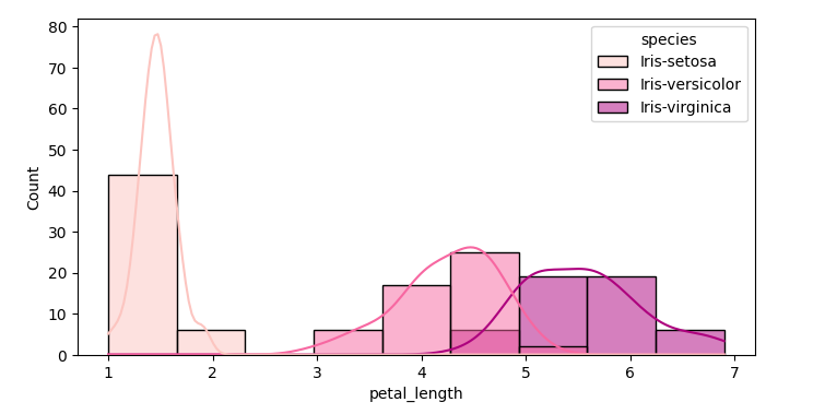
plt.figure(figsize=(8,4))
sns.histplot(data=df,x='sepal_width', kde=True, hue='species', palette='RdPu')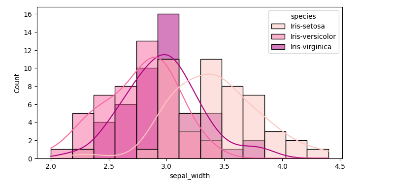
plt.figure(figsize=(8,4))
sns.histplot(data=df,x='sepal_length', kde=True, hue='species', palette='RdPu')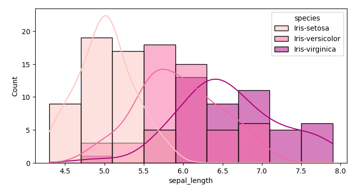
sns.pairplot(df, hue='species', palette='RdPu')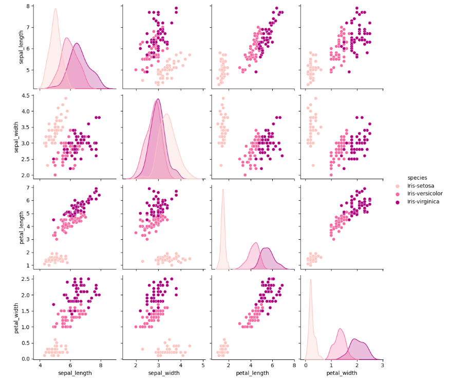
I will now prepare the data for the model training, encoding the species of Iris into a boolean variable
df_encoded = pd.get_dummies(df,drop_first = True)
df_encoded.head()
df_encoded = pd.get_dummies(df,drop_first =True)
df_encoded.head()
[17]:
| sepal_length | sepal_width | petal_length | petal_width | species_Iris-versicolor | species_Iris-virginica | |
|---|---|---|---|---|---|---|
| 0 | 5.1 | 3.5 | 1.4 | 0.2 | False | False |
| 1 | 4.9 | 3.0 | 1.4 | 0.2 | False | False |
| 2 | 4.7 | 3.2 | 1.3 | 0.2 | False | False |
| 3 | 4.6 | 3.1 | 1.5 | 0.2 | False | False |
| 4 | 5.0 | 3.6 | 1.4 | 0.2 | False | False |
and I drop one of the columns to avoid having multi-collinearity
X=df_encoded.drop(['species_Iris-versicolor', 'species_Iris-virginica'], axis=1)
y=df_encoded[['species_Iris-versicolor', 'species_Iris-virginica']]
I then proceed to splitting the data set, 80% for training and 20% for testing
X_train,X_test,y_train,y_test=train_test_split(X,y,train_size=0.8,random_state=42)Train the model
dtr=DecisionTreeRegressor(max_depth=3, random_state=42)Evaluating the model
dtr.score(X_train,y_train)0.9134209503031789
cross validate
from sklearn.model_selection import cross_validate
cross_validate(dtr, X_train, y_train, cv=5)
{'fit_time': array([0.00550103, 0.00378156, 0.00321126, 0.0033052 , 0.00319886]),
'score_time': array([0.00341892, 0.00229025, 0.00245166, 0.00244951, 0.00214362]),
'test_score': array([0.81286044, 0.97567621, 0.19327731, 0.79471509, 0.78635854])}
score on the test set
dtr.score(X_test,y_test)0.9991057076077319
Visualizing the decision tree
# plot tree
plt.subplots(figsize=(15,10))

plot_tree(dtr,feature_names=X.columns,filled=True);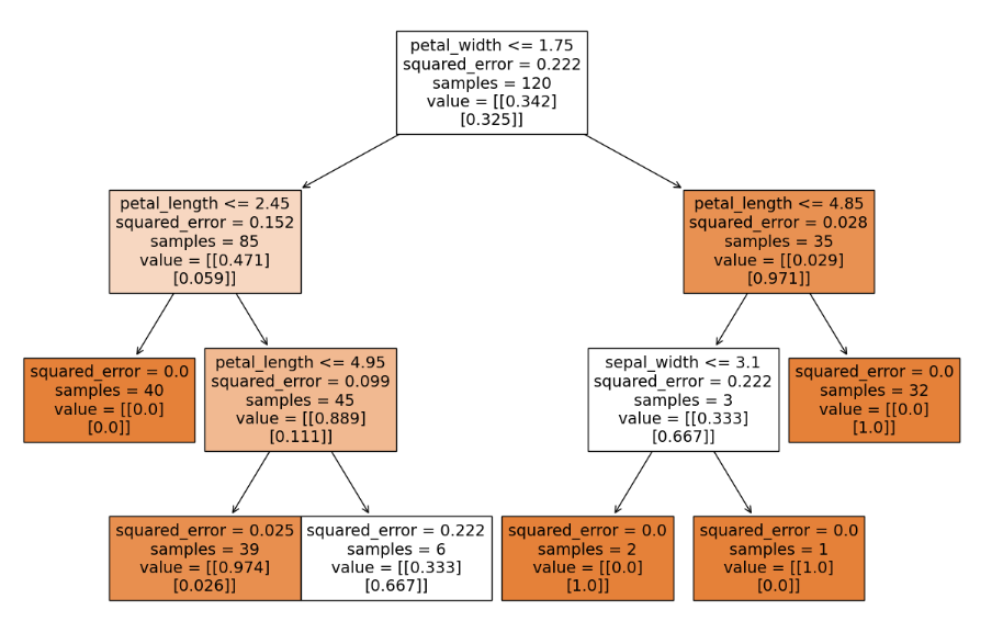
Leave a Reply